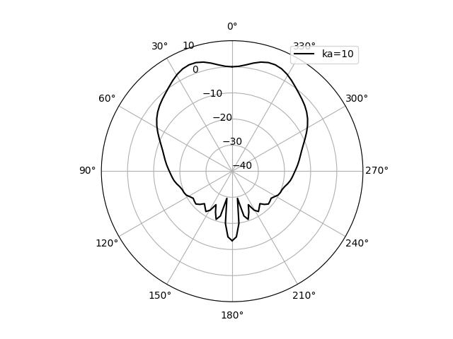
Oscillating cap of a sphere

import mpmath
from mpmath import sin
import numpy as np
import matplotlib.pyplot as plt
from beamshapes import cap_in_sphere_directivity
# sphinx_gallery_thumbnail_path = '_static//capsphere_ka-10.0_dps=50.png'

This model assumes a curved portion of a sphere (the ‘cap’) oscillates to produce sound. One cool thing about this model is that it produces somewhat uniform-ish beams that are frontally biased. For some ka values, the intensity is actually higher a bit off-axis (at higher ka’s).

Below, let’s reproduce an example to demonstrate these lobes that peak off-axis.

# if on Windows - the 'if __name__ == '__main__' is required.

if __name__ == '__main__':
    wavelength = (mpmath.mpf(330.0)/mpmath.mpf(50000))
    ka = 10
    k_v = 2*mpmath.pi/wavelength
    a_v = ka/k_v
    alpha_v = mpmath.pi/3
    R_v = a_v/sin(alpha_v) #mpmath.mpf(0.01)

    angles = mpmath.linspace(0,mpmath.pi,50)
    input_params = {'k':k_v, 'R':R_v, 'alpha':alpha_v}
    _, db_ratio = cap_in_sphere_directivity(angles, input_params)

    # save time by concatenating the same values for +ve and -ve angles

    plt.figure()
    a0 = plt.subplot(111, projection='polar')
    plt.plot(np.array(angles), db_ratio, 'k' ,label='ka=10')
    plt.plot(-np.array(angles), db_ratio, 'k' )
    plt.ylim(-40,10);plt.yticks(np.arange(-40,20,10))
    plt.ylim(-40,10);plt.yticks(np.arange(-40,20,10))
    a0.set_theta_zero_location('N')
    a0.set_xticks(np.arange(0,2*np.pi,np.pi/6))
    plt.legend()
    #plt.savefig('capsphere_ka-10.0_dps=50.png')